What Controls the Water Vapor Feedback?

Also available at: https://notesonclimate.substack.com/p/what-controls-the-water-vapor-feedback

Thanks to Andrew Williams and Daniel Koll for helpful feedback.

The water vapor (WV) feedback comes from the ability of a warmer atmosphere to hold more water vapor, which in turn lets less radiation escape to space. Intuitively, we’d expect the WV feedback to be largest where the atmosphere holds more moisture, and indeed models show the WV feedback ranging from roughly +3 Wm-2K1 (a strong positive feedback amplifying surface warming) at the equator to almost zero at the poles:

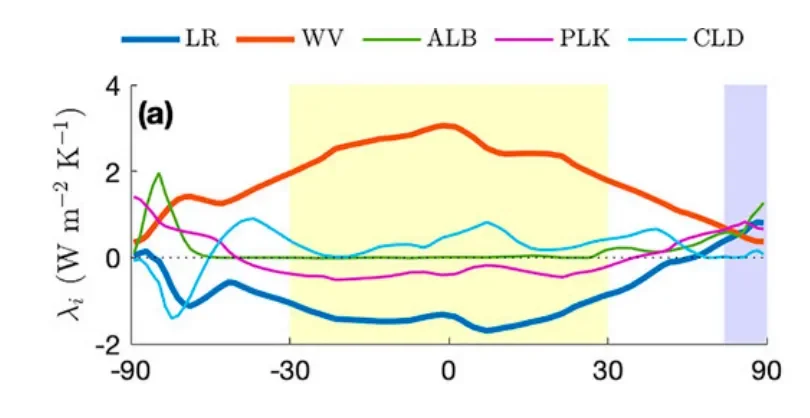
Figure: Latitudinally-varying feedbacks as calculated from CMIP5 simulations, adapted from Beer and Eisenman (2022). The red line shows the zonal-mean WV feedback.

The apparent link between moisture and the WV feedback makes sense at first glance, but it turns out to be misleading. In fact, the shape of the WV feedback is largely determined by surface temperature, rather than by how much water is in the atmosphere.

To see why, let’s simplify Earth’s longwave (LW) emission into a “partly-Simpsonian” model with two spectral regions:

(1) opaque wavelengths where water vapor is optically-thick, and

(2) a window region where water vapor is optically-thin.

In the opaque region, the emission to space comes from a WV emission temperature Th2o, while in the window region the radiation escaping to space is emitted at the surface temperature Ts. The total LW radiation emitted to space ( R ) is:

R = w σTs^4 + (1 - w)σTh2o^4,

where w is the fractional spectral width of the window and σ is the Stefan-Boltzmann constant.

The WV feedback is the change in R per unit change in column specific humidity (q), holding everything else fixed, multiplied by the change in q per unit surface temperature change:

λwv = dR/dq x dq/dTs,

or, in terms of the logarithmic derivative:

λwv = dR/dlnq x dlnq/dTs.

For simplicity, let’s now approximate the Clausius-Clapeyron relation by a fixed exponential:

q(T) = q(T0)e^ɑT,

where T0 is a reference temperature and ɑ is a constant. So dlnq/dTs = ɑ, and

λwv = ɑ dR/dlnq.

If ɑ is fixed, this means the geographic structure of the WV feedback comes from dR/dlnq.

So how does R depend on lnq? Going back to the expression for R, changing specific humidity could influence the window width w and the H2O emission temperature Th2o. As discussed in our 2023 paper, the window width depends linearly on lnq, so dw/dlnq is a constant (β). In other words, the narrowing of the WV window is more or less independent of temperature (hence of latitude).

Meanwhile, the water vapor emission temperature will be roughly the same at all latitudes. Here’s why: the emission to space comes from near where the WV optical depth equals 1, which occurs where there’s a certain mass of WV above. Under fixed relative humidity (RH), the WV mass at a given temperature is set by Clausius-Clapeyron, so we’d expect τ = 1 to be at the same temperature everywhere (~250-260K), even if not the same altitude. Hence Th2o is roughly independent of latitude.

Complications like variations in RH, pressure broadening, and other “non-Simpsonian” effects will cause some variation in Th2o, and I’ll return to some of these below, but these are too small to explain the geographic structure of the WV feedback.

This leaves the surface temperature Ts as the driver of geographic variations in the WV feedback:

λwv = ɑ dR/dlnq ≅ ɑ x dw/dlnq x (Ts^4 - Th2o^4) = ɑ x β x (Ts^4 - Th2o^4) ,

where ɑ, β and Th2o are all constant. In other words, λwv scales with the fourth power of the temperature difference between the surface and the water vapor emission level, and only Ts varies in space1. In the tropics, the temperature difference is large (e.g., 50K), while at the poles the difference is much smaller, or even zero. Furthermore, because both temperatures are raised to the fourth power, even small temperature differences translate into large variations in feedback strength.

To first-order, then, the geographic structure of the water vapor feedback is set by surface temperature. However, the two key approximations we made both damp geographic variation in λwv. First, in reality ɑ decreases at warmer temperatures, so dlnq/dTs is smaller in the tropics. Second, we showed in the 2023 paper that, rather than being fixed, the H2O emission temperature increases weakly with surface warming, roughly as Th2o ~ Ts^{1/4} (see discussion at bottom of p1932). This surface temperature dependence reduces the emission contrast Ts^4 - Th2o^4 ~ Ts^4 - Ts, which also damps geographic variations. We also left out RH, which matters both at the surface and in the upper troposphere, but isn’t a major driver of geographic variations (the subtropical RH minima don’t really show up in the WV feedback profile above).

It’s counterintuitive that the shape of the WV feedback depends on surface temperature rather than the atmosphere’s moisture content, but this is a good example of why using specific humidity as a state variable can obscure the physics of radiative feedbacks. Several papers have advocated for using RH-based feedbacks instead, as they give a much cleaner picture of what’s going on. In this framework, the radiative effects of WV increasing at fixed RH are absorbed into the Planck feedback (since WV just follows temperature), and only departures from fixed RH appear as a separate “RH feedback.” The surface temperature dependence of increasing WV at fixed RH then becomes intuitive: it’s baked into the reference Planck response.

1 At warm enough temperatures we have to account for emission from the WV continuum in the window region. This doesn’t affect the substance of the argument, but does damp the geographic variation. Since the WV continuum is optically thin even in the tropics, the emission temperature in the window is a weighted average of the surface and continuum emission temperature. You can see this in Figure 1 here.